The square law as an interception problem (ODEs, control and spacetime) - Part II
In Part I (discrete) the message was: the “square law” is not magic, it is a reachability condition with a time horizon. The board was \(\mathbb{Z}^2\), time was turns, and the “square” appeared because the king moves with the \(L_\infty\) metric.
In this Part II we take the continuous limit not to “approximate chess”, but to reveal the mathematical structure: pursuing a moving target, with bounded speed, before a deadline.
Guiding idea (in one sentence)
The king generates a reachable set that grows with time; the pawn traces a trajectory. Capturing is: “do they intersect before \(T\)?”
0 · Notation and three key concepts (without which this looks like witchcraft)
Before getting into equations, let’s clarify three words that will appear all the time:
ODE
An ordinary differential equation describes how a state changes with time: \(\dot{\mathbf{x}}(t)=f(\mathbf{x}(t),t)\). A “dot” means derivative with respect to \(t\): \(\dot{x}=\dot{x}(t)\).
Control
In many systems, there isn’t a unique dynamics: there is a family of dynamics depending on what you choose to do. This is modeled by introducing a variable \(\mathbf{u}(t)\) (“what you decide”) inside the ODE.
Norm and ball
A norm \(\|\cdot\|\) measures size/distance. The ball of radius \(r\) is the set \(\{\mathbf{v}:\|\mathbf{v}\|\le r\}\). With \(L_2\) the ball is a circle; with \(L_\infty\) it is a square.
The question that replaces “do I get there in \(n\) moves?” is: does there exist a time \(t\) such that I can be at that point while respecting my speed limit?
Mental translation
A discrete turn is like a “time budget”. When moving to continuous time, that budget is spread over an interval: you don’t jump, you move with a maximum speed.
2 · The king as a control system (ODE) and why \(L_\infty\) appears
Here \(\mathbf{u}(t)=(u_x(t),u_y(t))\) is the velocity you choose at each instant. To make this “the same king” as in the discrete model, we impose a speed bound that allows diagonal progress without extra penalty:
Why \(L_\infty\) and not \(L_2\)? Because in discrete chess a diagonal step costs the same as a straight one. In continuous time, that corresponds to allowing \(x\) and \(y\) to change “at the same time” up to the same limit, without making diagonals “more expensive”.
What \(\|\mathbf{u}\|_\infty \le v_k\) means physically
It means: “I can’t change \(x\) faster than \(v_k\), and I can’t change \(y\) faster than \(v_k\)”. Since you can push both at once, the extreme directions form a square of admissible velocities.
3 · The pawn: a simple ODE + a deadline
For the pawn we use the “clean” case: it moves straight, at constant speed \(v_p\):
Integrating that ODE is just “add velocity times time”:
\[ \mathbf{p}(t)= \begin{pmatrix} x_p\\ y_p + v_p t \end{pmatrix}. \]
And there is a time horizon: promotion. If promotion happens at \(y=y_{\text{promo}}\) (in chess, \(8\)):
\[ T=\frac{y_{\text{promo}}-y_p}{v_p}. \]
Why the deadline is the ingredient that “creates” the square law
Without a deadline, this would be “can I intercept at some infinite time?”. With a deadline, it becomes “can I intercept before \(T\)?”. That restriction turns a time pursuit into a spatial initial condition.
4 · The king’s reachable set: the object that replaces “distance”
The general solution for the king (integrating the ODE) is:
This is already the “square law” in its pure form: at fixed time \(t\), the king covers a square. The discrete one was the same square, just pixelated.
How to read \(\|\mathbf{x}-\mathbf{k}_0\|_\infty\le v_k t\)
It means that both in \(x\) and in \(y\) you can correct at most \(v_k t\). It is the simultaneous condition: \(|x-x_k^0|\le v_k t\) and \(|y-y_k^0|\le v_k t\). That is a square centered at \(\mathbf{k}_0\).
5 · Capture = “does the pawn’s trajectory enter the reachable set?”
Capture means that at some instant \(t\in[0,T]\) the king and the pawn coincide:
This is exactly the same logical pattern as in the discrete case
Part I: “\(\exists\) turn \(t\)” such that “discrete distance \(\le t\)”. Part II: “\(\exists\) time \(t\)” such that “distance induced by speed \(\le t\)”. The objects change, not the logic.
6 · From a vector condition to inequalities (math-heavy, but chewed)
Substitute the pawn’s explicit trajectory: \(\mathbf{p}(t)=(x_p,\ y_p+v_p t)\). To separate horizontal from vertical, define:
\[ a := |x_p - x_k^0|, \qquad b := y_p - y_k^0. \]
Comment: \(a\) is lateral separation (always nonnegative). \(b\) is vertical separation with sign: if \(b>0\), the pawn is above; if \(b<0\), the king is above.
The capture condition becomes:
\[ \|\mathbf{p}(t)-\mathbf{k}_0\|_\infty \le v_k t \quad\Longleftrightarrow\quad \max\big(a,\ |b+v_p t|\big)\le v_k t. \]
That inequality with \(\max\) splits into two simpler ones:
\[ a \le v_k t \quad\text{and}\quad |b+v_p t|\le v_k t. \]
The first is immediate:
\[ t \ge \frac{a}{v_k}. \]
The second is an absolute value; open it as a “double inequality”:
\[ -v_k t \le b+v_p t \le v_k t. \]
Subtract \(v_p t\) on all three sides:
\[ -(v_k+v_p)t \le b \le (v_k - v_p)t. \]
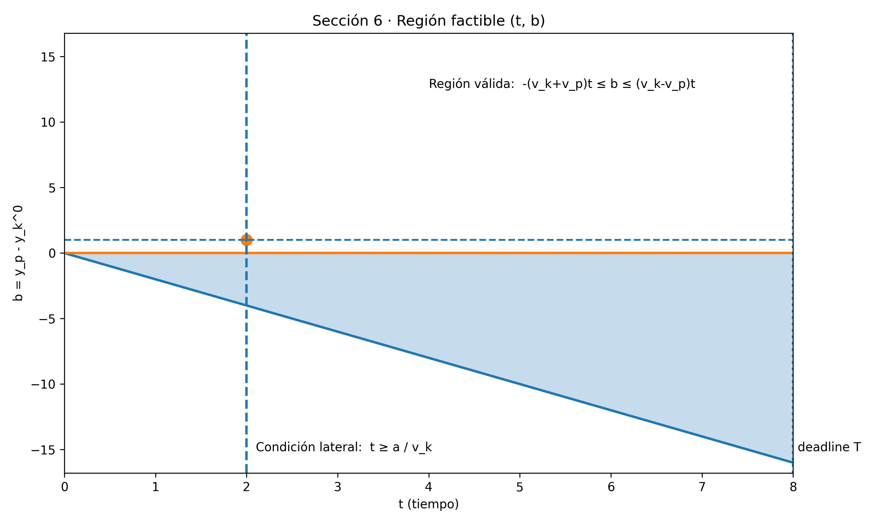
Plot · Feasible region in the (t, b) plane
The shaded strip represents the pairs \((t,b)\) satisfying \(- (v_k+v_p)t \le b \le (v_k-v_p)t\). The dashed vertical line marks the lateral condition \(t \ge a/v_k\).
Interpretation: for a given \(b\), capture exists if its horizontal line intersects the shaded region at some \(t\) within the horizon.
Here appears the real dynamic content. The expression \(v_k-v_p\) is the king’s “speed advantage” over the pawn.
Intuitive reading of \(\;b \le (v_k-v_p)t\)
If the pawn starts ahead (\(b>0\)), to catch it the king must be able to “erase” that lead. That is only possible if \(v_k>v_p\) (positive advantage). If \(v_k=v_p\), the best you can do is not get worse, but you can’t close the gap.
7 · Recovering the square law (chess case) without hiding what’s going on
With \(v_k=v_p\), the vertical inequality \(b \le (v_k-v_p)t\) becomes:
\[ b \le 0. \]
This is a consequence of the idealized continuous model: if both have the same speed limit, the king cannot eliminate a positive vertical disadvantage “in the long run”. (In real chess, the fact that the pawn does not capture forward, and that the king can take “shortcuts” via specific squares, adds nuances; here we are isolating the basic geometry.)
The operational rule used as a heuristic —and matching Part I— can be written as:
\[ \|\mathbf{p}(0)-\mathbf{k}_0\|_\infty \le T. \]
The condition \(\|\mathbf{p}(0)-\mathbf{k}_0\|_\infty \le T\) says the king is inside the \(L_\infty\) ball of radius \(T\) around the pawn. But the \(L_\infty\) ball is a square. So “being inside the square” is exactly that inequality.
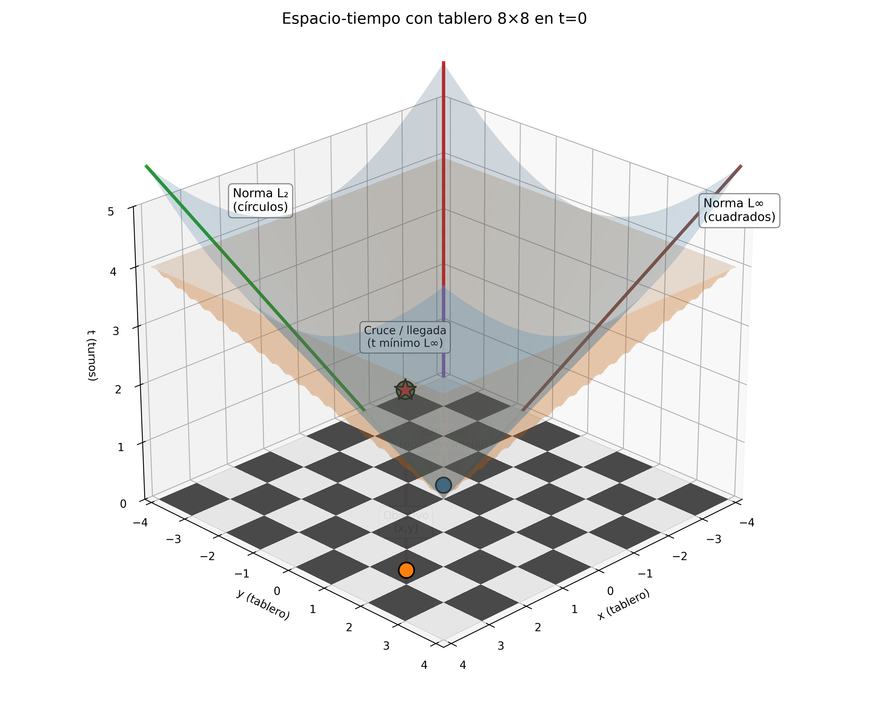
8 · Continuous causal cone: the correct 3D mental picture
Geometric visualization in spacetime
The plane t=0 is the board. The pyramid represents the \(L_\infty\) norm (king movement) and the circular cone the \(L_2\) norm.
In Part I we talked about a “discrete causal cone” by stacking reachable regions per turn. In continuous time the cone is literal: the set of all points \((\mathbf{x},t)\) the king can reach at time \(t\).
If you cut the cone \(\mathcal{C}\) at time \(T\), you get \(\mathcal{R}_k(T)\), a square. The pawn’s “square” is the spatial projection of that idea: “at time \(T\), are you inside?”.
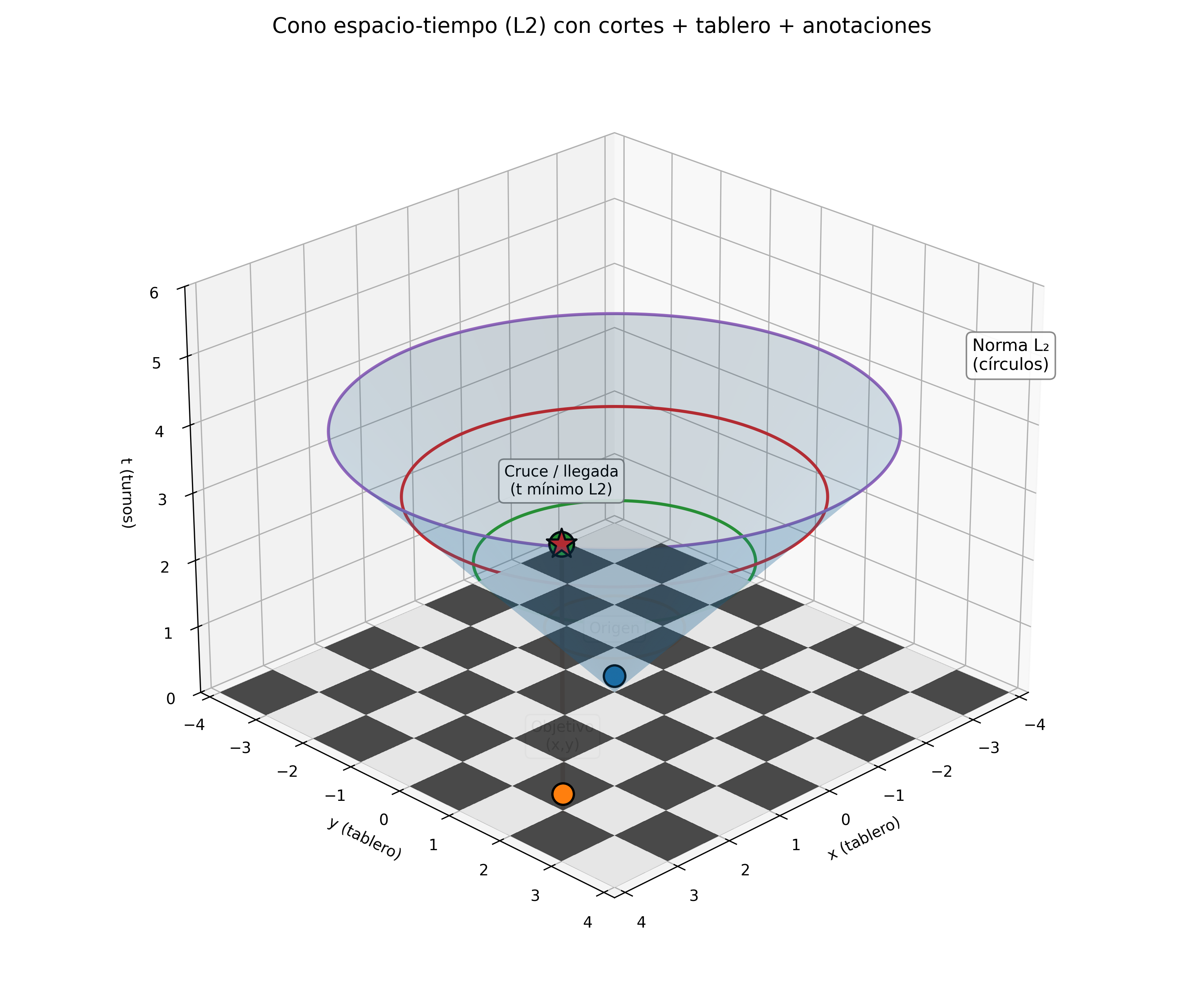
Continuous causal cone of the king
Each horizontal slice represents the reachable set at fixed time under the \(L_2\) metric. The circles show radial growth of the causal front.
The reachable front grows linearly with time: \( \|\mathbf{x}-\mathbf{k}_0\|_2 \le v_k t \).
9 · Bonus: from ODEs to Hamilton–Jacobi / Eikonal
Up to here we only needed ODEs. But there’s another way to look at the same thing: instead of pursuing a specific trajectory, describe the minimum time to reach any point \(\mathbf{x}\).
This \(V\) satisfies an anisotropic Eikonal-type equation associated with Hamilton–Jacobi. One way to see it (without the full theory) is that the slope of \(V\) is limited by the maximum speed, and the dual norm that appears in the gradient is \(L_1\).
\[ \|\nabla V(\mathbf{x})\|_1 = \frac{1}{v_k}. \]
If instead of \(V\) you describe a front \(\phi(\mathbf{x},t)=0\) (a “propagating boundary”), its evolution satisfies a propagation PDE:
In isotropic propagation (\(L_2\)) the front grows as circles. Here the front grows as squares because the metric induced by the control is \(L_\infty\). Same story, told with PDE language.
Summary: in discrete time we drew a square; in continuous time we derive it as a slice of a reachable cone. The equations add an important detail: the square is not an arbitrary heuristic, but the reachable set of a dynamical system with control bounded in the \(L_\infty\) norm.
If in Part I the argument was “discrete distance \(\le\) remaining time”, here it is “speed-induced norm \(\le\) deadline”. The square law is the same inequality, seen at two resolutions.